Low Volume PCB Assembly: How Many to Build First?

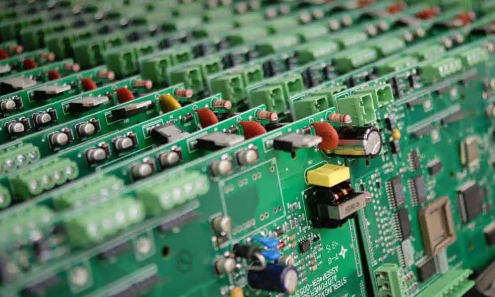
When dealing with low volume PCB assembly, the process will often be guided by the variable quantities of products involved (in this case, assembled circuit boards) and the fact that designs may need to change frequently to accommodate new technology or processes being tested during this time. This type of production may be helpful in terms of introducing a new product to market, evaluating the marketability of multiple product types, providing spare parts for products whose use or volume has diminished, and transitioning from an uncertain level of demand to a more established level of demand.

The term “low volume” is subjective and will vary between different manufacturers depending on their individual business models, as well as how many different types of products they manufacture. The key to determining what “low volume” means for your company is to first establish the risks and variables associated with your product and design until it reaches production. Once you have identified these variables, establish how many assembled circuit boards you will need in order to answer engineering and production questions, support multiple internal teams needing to use the same product, and preserve any units intended for destructive testing or retention. Finally, avoid exposing your entire order to any revisions that have not yet been authorized for release. This allows low-volume assembly to be used as both a lower-quantity ordering approach and a means of managing product development from design through a repeatable production process.

Key decision rules

• Do not use a manufacturer’s quantity band as the only definition of low volume. The same quantity can be defined as a prototype, pilot, repeat production order, or high-mix configuration problem depending on the manufacturer and the production context.
• Demand, material purchased, assembled quantity, and deliverable quantity can all differ from one another. The assembled quantity should be sufficient to answer the required engineering and production questions.
• Define what evidence is needed to classify the result as Continue, Hold, or Re-spin prior to commencing assembly, and identify who has the authority to approve the remaining quantity of products.
• A small clean sample only represents the product that passed inspection or testing under the stated conditions, not the total population from which it was taken.

What Is Low Volume PCB Assembly?

Low volume PCB assembly comprises all the same basic production methods as higher-volume PCB assembly: controlled product data; component preparation; solder paste application when applicable; automated or hand placement; reflow or selective soldering; visual inspection; programming; testing; rework control; and traceability. It differs primarily with respect to the production economics of the order and the tolerance for changes. Fixed setup effort will be spread over fewer units, design revisions are more likely to occur, material may be procured in quantities that do not match the assembly quantity, and the engineering group will frequently want to use boards prior to receiving the total order.

Thus, low volume is not limited to prototype assembly. A prototype is generally optimized to gain knowledge about either the functional capabilities of a product or design feasibility. A low volume order may utilize released drawings, controlled BOMs, production equipment, defined acceptance criteria, and repeatable test methods. Low volume production can also serve as an intermediate stage in NPI, and it may be the normal method used to manufacture high-mix or longer-lifecycle products with demand that never justifies high-volume economics.

What Counts as Low Volume?

There is no standard number available from the PCB industry that categorizes PCB assemblies as “low volume.” Supplier-published definitions commonly range from tens or hundreds of units up to the low thousands; these ranges are generally commercial shorthand, not a recognized engineering threshold. A quantity of 200 assemblies could represent either a controlled pilot run for one type of product or an established recurring production run, depending on the level of fixed effort repeated, the maturity of the design and test process, the number of product variations sharing the same resources, and the level of inventory risk the customer can accept.

When Does Low-Volume PCB Assembly Make Sense?

New Product Introduction and Pilot Production

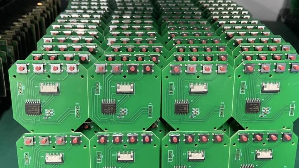
One point at which low volume PCB assembly is beneficial is during the NPI and pilot production stages. During the NPI phase, while the prototype may function correctly, there may still be manufacturing, programming, mechanical, thermal, and test-related risks associated with the assembly of multiple production units. Low-volume pilot production allows engineering and operations to verify repeatability without incurring the full demand risk due to uncertainty surrounding product revisions.

To have a successful low-volume PCB assembly pilot production run, identify these concerns before ordering the pilot volume: power sequencing, firmware communications, connector access, enclosure fit, thermal characteristics, calibration, fixture accessibility, and repeatability can all require different quantities of units. For example, while connectors may seat properly on a prototype bench-assembled product by hand, the tolerance stack created by production placement and reflow processes may not allow the connector to seat properly when assembled on a production basis. This assembly problem may only present itself when several units go through the same fixture back to back. The low-volume pilot run should end with an approved release or decision point rather than the subjective conclusion that “the boards worked.”

Market Validation

Although a product may be technically stable, demand for that product may still be uncertain. Low volume production in this case mitigates the risk of excessive inventory on hand. As a result, the engineering focus may switch from locating design flaws to validating field configuration, packaging, programming, serviceability, and customer acceptance while minimizing large inventory purchases. The quantity should represent near-future anticipated demand, potential replacement requirements, supply continuity, and the cost of another manufacturing setup.

Therefore, the market validation process is not a justification for arbitrarily changing configurations. The unit being delivered must have a defined product configuration, a defined firmware state, a defined test method, and a defined disposition route to verify that the feedback received in the field corresponds to the proper revision of the unit. An example of this risk is a batch of 100 units manufactured using a demand forecast of 100 units but selling only 30. If a firmware revision is released before the remaining units are delivered to the customer, the remaining 70 units require a documented method for reflashing or scrapping before they are shipped, rather than deciding whether they should be reflashed on a unit-by-unit basis at the time of fulfillment.

High-Mix and Multiple Configurations

In high-mix production with multiple configurations, a single manufactured bare PCB might be assembled based on multiple BOMs (bills of material), DNP options (do not populate), firmware images, connectors, regional features, test programs, or product features. As such, the low volume nature of manufacturing these products creates a configuration issue as well as potentially a quantity issue. A lot of 100 bare boards is not necessarily the same as one assembly lot of 100 units when 40 are assembled with one BOM, 30 with one set of firmware and connectors, and 30 are left unpopulated to support an option later on. Variant-specific fixtures, programming, acceptance criteria, and supply-chain shortages, such as unavailable components, can require separate allocations even if the bare-PCB geometries are identical.

Long-Lifecycle, Low-Demand Products

Some industrial, laboratory, infrastructure, aerospace, medical, or specialized B2B products will not move into high-volume production due to their low annual volume projections or because they will remain customer-specific in their configurations. Therefore, low volume may remain their normal production state over the entire lifecycle rather than serving as a temporary transition stage. The priorities associated with controlling the production of these products also change accordingly; approved alternate parts, component lifecycle, inventory retention, revision traceability, reproducible tests, repair information, and restart readiness may take precedence over cost reductions related to unit production volume.

When another repeat order is placed years later, it is essential that the manufacturer and its customer do not depend on memory for the previous PCB, BOM, placement data, programming instructions, fixtures, acceptance criteria, and approved deviations. The PCB, BOM, placement data, programming instructions, fixtures, acceptance criteria, and approved deviations used to produce a product must identify what was used in the last production run and what has changed since then.

A common example of failure occurs when a key component becomes obsolete between orders and an approved alternate part is used on the restart, but the BOM revision and test limits are not updated to reflect the change. As a result, the next repeat order may restart from records that no longer match what was actually built and shipped.

Prototype vs. Low-Volume vs. High-Volume PCB Assembly

The boundaries overlap. There is no reason that a five-unit assembly run using released production tooling cannot be more mature than a 200-unit engineering pilot run. Product state and the decision-making purpose matter more than the label attached to the quantity.

Cost, DFM, and Component Readiness Before Assembly

Fixed Setup and NRE Cost

For low volume assemblies, since fixed setup costs are amortised over fewer total assemblies, the cost per assembly is usually higher than for high volume assemblies. The fixed setup effort or NRE effort is usually project-specific and can include preparation of solder paste stencils, programming setup, machine programming and verification, tooling, verification of the first assembly, assembly documentation, material handling, and line setup. Therefore, there is no reliable universal “typical” setup fee; it is usually specific to the supplier and the project.

A useful method of calculating the cost associated with fixed setup costs or NRE costs for an assembly is as follows:

Fixed-cost contribution per PCBA = total fixed setup/NRE cost ÷ assembled quantity

The following numbers are an illustrative planning example, not a supplier quotation. If fixed setup and NRE total $180:

A unit’s price should typically decrease as its quantity increases; however, the fact that a unit’s cost can decrease due to volume does not prove that 100 assembly units are less costly for the project. When a pending (unresolved) change renders 100 assembly units invalid, the setup cost savings can be significantly less than the costs associated with rework, scrap, replacement material, and rescheduling caused by assembling too many units too early.

DFM, DFA, and DFT

DFM, DFA, and DFT should always be reviewed prior to production runs of any size. Multiple small production runs can actually compound the costs associated with unnecessary setup and rework when the same problem is recreated each time the product is produced. When reviewing the released design data, you need to consider three parts of the DFM, DFA, and DFT processes.

DFM—Will the footprints, pad layouts, component spacing, polarity, fiducials, panelization, component clearances, thermal features, and manufacturing constraints be accommodated by the manufacturing process selected?

DFA—Can the components be assembled, soldered, inspected, cleaned, handled, or reworked without requiring additional manual operations, creating access conflicts, or causing confusion with other variants?

DFT—Will the programming connections, test points, fixture access, measurement limits, diagnostic coverage, and data capture be appropriate for making the required decisions?

A DFM or DFT review will assist you in identifying discrepancies in footprint layouts, inadequate test access, and problems with panel layouts or clearances before they occur throughout the production run. A DFM or DFT review does not identify failure modes that may occur only when a board is subjected to load, thermal cycling, or field handling. It therefore cannot by itself support or justify either the reliability of the population being tested or the remaining quantity. Those claims must still be based on appropriate test evidence and release criteria.

BOM, MOQ, and Component Availability

The assembly quantity and component purchase quantity can vary significantly. For example, a 50-unit assembly may require not only a complete reel of components, but also a minimum purchase from a distributor, as well as extra components for feeder setup, spare parts, or a lifetime purchase of a component where there is limited availability. Approved alternate components can help eliminate delays when the product definition and qualification rules permit their use.

Customer-supplied parts raise additional questions regarding incoming condition, quantity loss due to handling, storage, ownership, and ultimate disposition. Some moisture-sensitive devices may require controlled storage and handling if assembly pauses between production batches.

Before ordering any spare bare boards and components, it is important to confirm whether they will continue to remain under the customer’s ownership, whether the parts can be stored under the proper conditions, what the costs are for restarting the production line after pausing, and whether a quantity that has been paused can be resumed without repeating programming, verification, inspection, or material preparation. A low quantity of parts to be assembled does not always equate to a low commitment of materials.

How Assembly Technology Changes Low-Volume Planning

The term low volume should not imply that the assembly method will necessarily be manual assembly. Low volume production can effectively utilize automated SMT placement and controlled reflow processes in instances where the benefits of setup, component presentation, and quality warrant these processes, even at low quantities. Increased labor sensitivity and greater importance of operator instructions are also evident in the use of mixed technologies, such as through-hole insertion, manual soldering, press-fit operations, wire attachment, or selective soldering.

Packages such as BGAs and QFNs can also significantly impact inspection strategies because important solder features are hidden from view during inspection. The primary question when using either SMT or through-hole technologies should centre around what specific operations are going to add fixed setup time, manual variability, special inspection requirements, or fixture requirements to the overall quantity and configuration being produced.

How Many PCBAs Should You Assemble First?

To answer this question, establish how many PCBAs you will need to assemble first so that you have enough units to close the set of named questions that you have established. However, do not assemble more than the unresolved design can safely expose. The amount of PCBAs that you decide to assemble will depend on the objectives you have established for “learning” and “release” purposes. In the case of proof-of-function assemblies, as well as pilot and market-validation runs, you may be using similar quantities. Still, the type of evidence and stop rules used during the assembly of these materials will vary greatly.

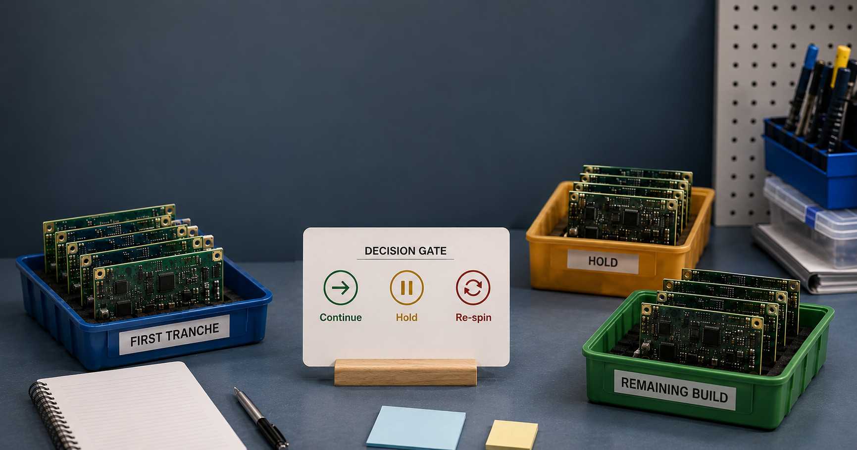
The design review process can eliminate preventable errors from the units and design features it covers, whereas conclusions about what it does not cover must still be determined by assembled and tested hardware.

Once you have established the questions—such as power-up, firmware communication, mechanical fit, thermal behavior, analog or RF performance, fixture access, pre-compliance screening, and repeatable assembly—their intended uses, timing windows, and whether they require concurrent, modified, environmental, or destructive specimens, you will be ready to select the quantity; a price break cannot replace that decision logic. Each planned assembly quantity will be a controlled fraction of the planned demand to be manufactured. Therefore, it cannot automatically be classified as an “engineering sample,” “production qualification,” “formal acceptance sample,” or “first article.”

Split Total Demand Into Usable Board Allocations

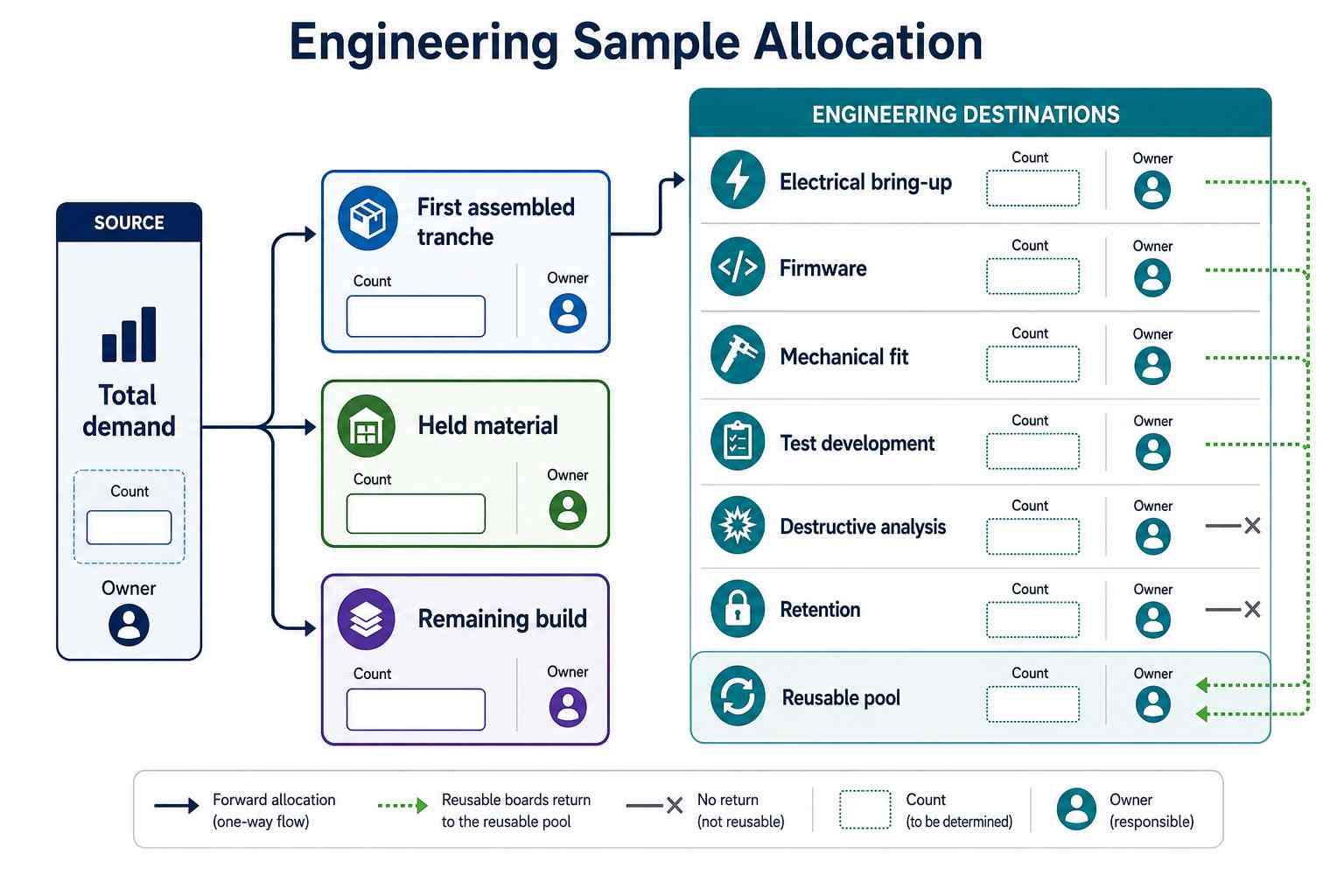
Total demand (the amount of product required), total materials purchased (the amount of material purchased), initial assembled quantity (the amount of product that you will assemble), and total deliverable quantity (the number of products that are to be delivered) all represent different numbers, and it is important to separate each number from the others before selecting the initial assembled quantity. Doing so ensures that the contractual total will not unintentionally become the basis for establishing the engineering sample plan and enables you to identify the assemblies that may return to the shared pool following testing.

Reuse works only when time and physical state allow it. An assembly may move from electrical bring-up to firmware development and then mechanical fit; however, it cannot meet simultaneous deadlines. Elements like coating, wire modifications, connector wear, thermal stress, cutting, and destructive analysis can permanently remove an assembly from the common pool. Furthermore, variant-specific fixtures and programs may also require separate allocations despite a shared bare-board design.

A Practical Quantity Planning Example

Our example requires two units for electrical bring-up, three concurrent firmware units, two units for mechanical fit, two units for destructive use, and one unit held in reserve. If we simply add all of the units required by the project, we would need ten units. However, we can eliminate duplicate requirements and determine the actual number needed using timing and scheduling factors.

After successful bring-up, if firmware work is completed before mechanical fit, then the peak reusable demand will be three units. Thus, we can get to our starting quantity as three reusable units + two destructive units + one reserve unit = six units before planning for contingencies. If it is necessary for three firmware units and two mechanical fit units to operate at the same time, then the peak reusable demand will increase from three to five. Therefore, the total quantity required for this project will be at least eight units before adding contingencies.

Planning model: initial quantity ≈ peak concurrent reusable demand + destructive units + reserved units + justified contingency

This planning model is not an industry standard. It forces the team to define its assumptions regarding quantity: concurrency, reuse, destructive work, retention, and accepted contingency.

What Makes a Smaller Initial Batch Worth the Extra Setup?

For a small batch size to be worthwhile, the reduced change and scrap exposure must outweigh the costs associated with reopening production, waiting, and idle engineers. In this regard, the trade-off works both ways: a small batch size can protect expensive boards and scarce components from potential redesigns. However, if an additional setup interrupts a critical integration sequence, the overall cost of the additional setup could exceed the potential redesign protection.

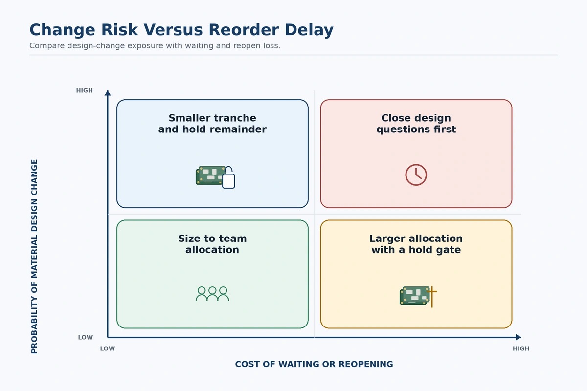
The cost of over-assembly is the exposure of bare boards, components, placement, soldering, programming, coating, rework, and schedule to one unresolved revision. The cost of under-assembly is the exposure to repeated setup, material handling, shipping, queue time, fixture downtime, and engineering team members waiting for usable hardware. Unit price alone does not represent the total project cost.

Non-recurring and fixed setup costs can be included within this trade-off. Starting a separate setup is likely to cause a recurrence of programming, verification, logistics, material preparation, or line setup. The time required to reopen any of those activities will depend on the current project and must include differences in component reservation, manufacturer’s capacity, tooling availability, shipping requirements, and approval delays for each project.

Match Inspection and Testing to the Decision

Inspection and testing procedures must be selected based upon “WHAT MUST WE PROVE?” rather than upon a generic “checklist.” Different claims can be supported by visual acceptance, hidden-joint inspection, circuit connectivity testing, functional operation testing, process evidence, reliability evidence, and regulatory compliance evidence. A testing procedure may be appropriate to support a reliability claim or reliability qualification, but may not demonstrate compliance with all design specifications.

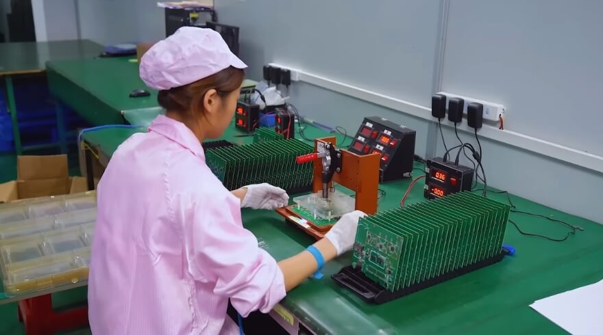
The IPC Class 3 classification is not automatically given to low-volume production; apply the correct end-use product class, workmanship criteria, and any customer and contractually required standards. The criteria established by IPC-A-610J address acceptability after assembly, while soldering process and material requirements are addressed by J-STD-001J. While they are related, the two documents cannot be interchanged.

Set Continue, Hold, and Re-spin Rules Before Assembly

The initial quantity creates value only when all required checks lead to permitted subsequent actions. The Continue, Hold, and Re-spin rules should be defined prior to starting the assembly process, and the authority for approving actions should also be defined. If these actions are not defined ahead of time, several usable boards may trigger the remaining quantity even while unresolved anomalies, workarounds, or revision mismatches invalidate the intended evidence.

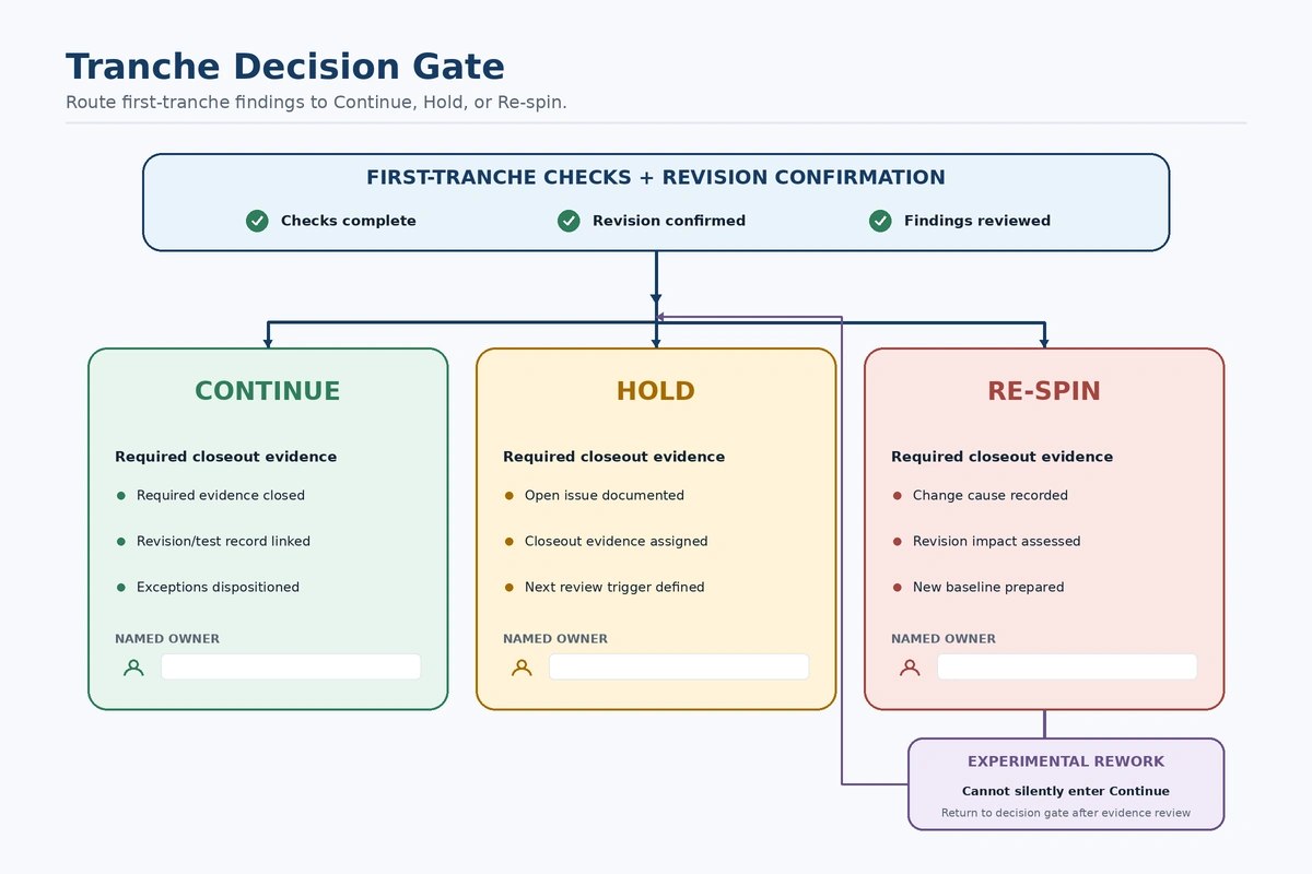
Rework is evidence that an issue occurred, not automatic release. Examples include the use of a fly wire to bridge a connection, using a laboratory substitute for a part in order to continue testing, changing the test limit of a test scheme, or using a manual workaround. In each case, the product may have been made functional for the experiment, but it does not define the manufacturing standard for the remaining parts.

The product may be classified as an experiment, approved deviation, or design change. If the remaining quantity of product cannot reproduce the accepted state under controlled instructions, the “Continue” process is not available even though the modified product functions.

A formal sampling scheme can be used as an analogy to the PCBA release process, rather than as a universal PCBA release rule. NIST describes acceptance plans with outcomes of acceptance, rejection, or additional sampling, including single, double, multiple, and sequential acceptance plans. Engineering release decisions utilize different project-specific criteria for the decision to continue with production.

What Does a Clean Small Sample Actually Prove?

A clean sample simply proves that the samples that passed inspection actually passed the inspections performed. A clean sample does not ensure that the population has a low defect rate, that the samples have long-term reliability, regulatory compliance, or that they will be capable of being manufactured at high volumes under conditions that were not examined. Once the parameters for the population definition, inspection object, testing method, testing configuration, and environment are defined, the ability to infer beyond those conditions from a clean sample is limited.

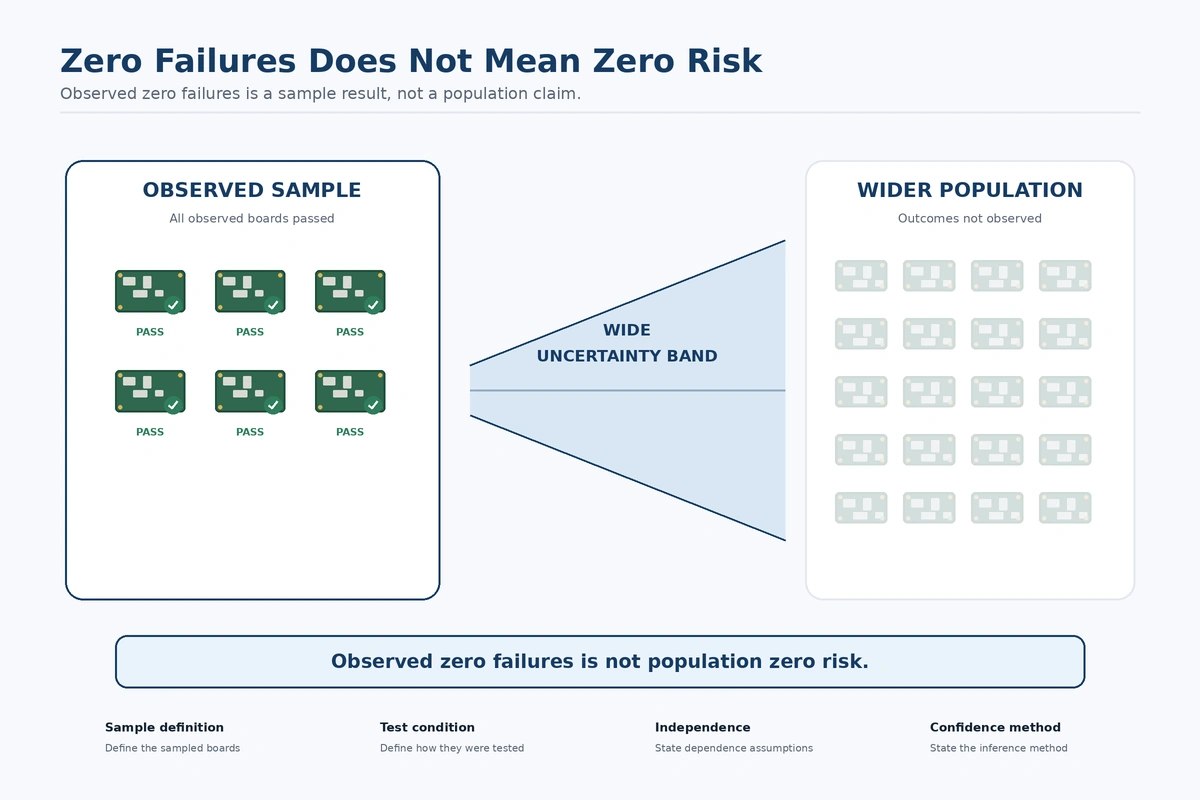
Although NIST treats acceptance sampling as a methodology for determining whether a lot is accepted or rejected, it does not consider acceptance sampling to be a direct indicator of the population’s defect rate. The risks that a producer and consumer assume when using acceptance sampling depend on the acceptance sampling plan used and the quality assumptions related to the product. The lack of any observed failures still leaves uncertainty, particularly when the sample size is small or failures are very rare. For rare failures, it may be more appropriate to use an exact binomial confidence method as opposed to a symmetric normal approximation. Without a defined confidence level, a defined population, an independence assumption, and a documented pass/fail event, a universal percentage is false precision.

ISO 2859-1:2026 defines AQL-indexed, lot-by-lot sampling schemes for inspection by attributes, including single, double, and multiple forms. An AQL value does not permit the intentional manufacture or shipment of that percentage of defective product. The contract, lot definition, type of inspection, switching rules, and the established risk plan dictate how the standard is to be applied.

An aerospace FAI is distinct from the above activities. AS9102C establishes requirements for performing and documenting FAI when FAI is required. Aerospace FAI is not necessarily the definition of all commercial initial low-volume products. The engineering sample, formal acceptance plan, and contractually required FAI should not be considered interchangeable unless explicitly linked.

How Should Evidence Carry Into the Remaining Assembly?

All evidence must be connected to the remaining assemblies. Each product revision, material status, programming state, inspection object, test configuration, exception, and approval must indicate the conditions that were evaluated and the quantity authorized to proceed. A passing unit with an undocumented patch, alternate material, modified fixture, or altered limit cannot serve as the basis for untouched units merely because the modified unit passed.

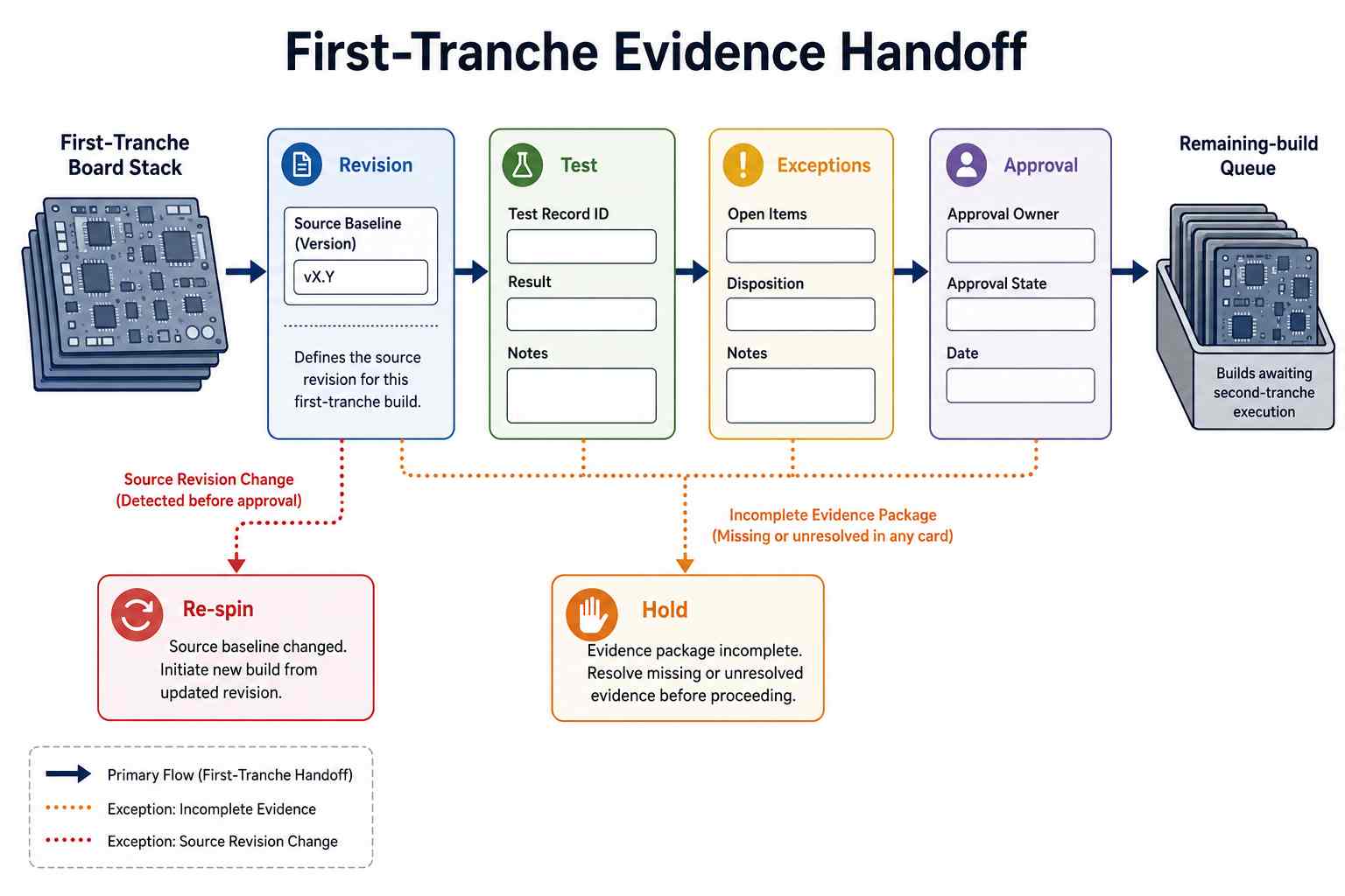
IPC-1782B provides a risk-based framework for traceability in manufacturing and throughout the supply chain. Traceability depth should correspond with the product, contract, and agreed risk. This allows enough linkage to provide evidence of which state was evaluated, what was changed, who accepted the change, and what quantity can proceed to the next stage. If an initial batch contains an undocumented patch, an unapproved substitute, a changed limit, a fixture revision, or an unexplained failure that could invalidate the released configuration, the remaining quantity must remain on Hold.

When Should Low-Volume Production Scale?

Scaling should be based on evidence and not simply awarded because you completed a small order. The ability to scale should be based on whether the product definition is stable, required testing has been released and is repeatable, open anomalies are dispositioned, sourcing is sufficiently controlled, assembly and inspection processes have demonstrated repeatability, and there is demand to justify the additional inventory exposure. The exact threshold will vary based on the project.

Low volume may also remain a valid long-term strategy. High-mix configurations, limited annual demand, customer-specific options, long service lives, constrained components, or lot-specific approvals can make repeated small production more justifiable than moving to a high-volume conversion. In these cases, the improvement target is not always to produce higher volume, but instead may be to achieve a more repeatable restart, cleaner configuration control, stronger test evidence, less variability in manual assembly processes, and better component continuity.

A defensible low-volume plan can trace any assembled unit back to the question it was intended to answer and the evidence that allowed the remaining quantity to proceed.

Related SUGA-PCBA Resources

SUGA-PCBA low-volume assembly capabilities

SUGA-PCBA inspection and test capabilities